XLOOKUP with Dropdown in Excel — The Smartest Lookup Trick You Need Today

If you want fast, dynamic and error-free lookups, then learning XLOOKUP with Dropdown in Excel is one of the smartest tricks you can add to your workflow. Whether you are building dashboards, MIS reports, financial models, salary sheets or product search tools, this combination makes your Excel files interactive, responsive and highly professional.

In this guide, you’ll learn how to set it up in less than one minute — exactly as shown in the script:

Create a dropdown → Apply XLOOKUP → Change dropdown → Result updates instantly.

Let’s unlock this powerful Excel skill.

---

---

What Is XLOOKUP with Dropdown in Excel?

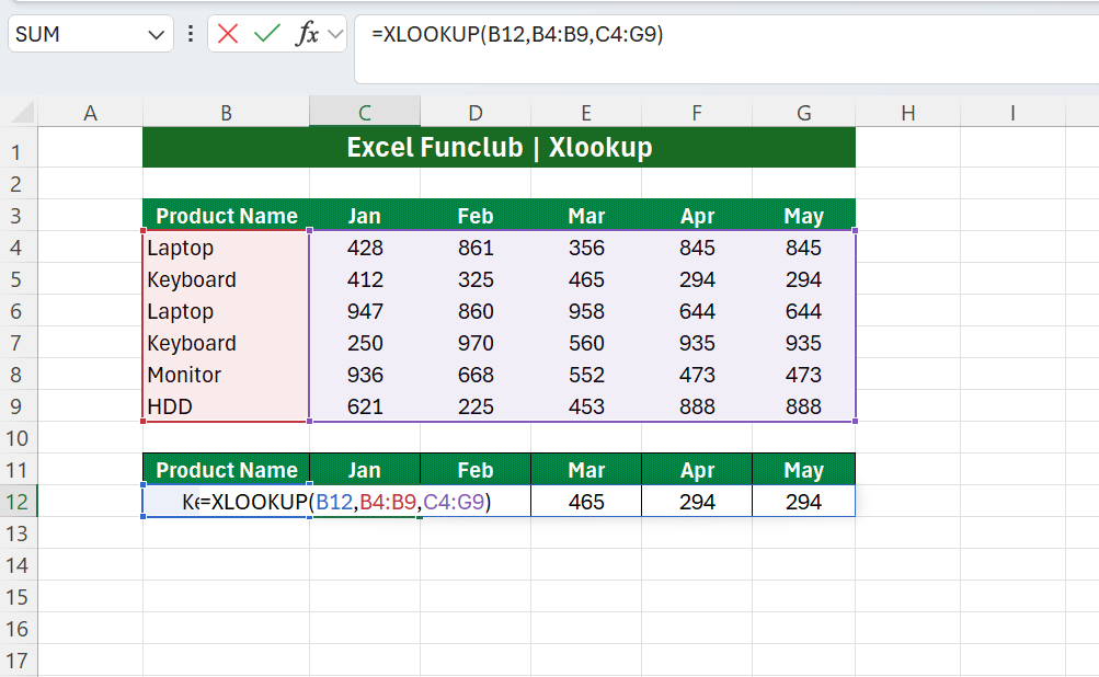
XLOOKUP with Dropdown in Excel simply means using a Data Validation dropdown list as the lookup input value for the XLOOKUP formula.

So instead of typing search values manually, you select an item from a dropdown, and Excel automatically retrieves the matching result.

This technique:

• reduces errors
• makes dashboards dynamic
• saves time
• makes reports more user-friendly

➤ Think of it as “searching without typing.”

---

Why XLOOKUP with Dropdown in Excel Is a Game-Changer

Here are some powerful benefits:

1. Super Fast Lookups

You no longer need to manually enter employee names, product codes, or IDs. Just pick from the dropdown and Excel does the rest.

2. Professional Dashboard Experience

Dropdown + XLOOKUP = interactive reports that feel automated.

3. Zero Errors

Manual typing mistakes? Gone!

4. Perfect for Repetitive Tasks

MIS teams, HR, finance, sales analysts — everyone gets speed + accuracy.

---

Step-by-Step Guide: How to Use XLOOKUP with Dropdown in Excel

(Your complete script converted into a full professional tutorial)

Below is the exact sequence from your Shorts script, expanded with explanations:

---

Step 1: Create a Dropdown Using Data Validation

Press:

Alt + A + V + V

This keyboard shortcut directly opens Data Validation → List.

Now:

• Select the cell where you want your dropdown (for example, C2).
• Choose “List”
• In Source, select your lookup values (e.g., A2:A20).

Your dropdown is ready!

---

Step 2: Start Writing the XLOOKUP Formula

In the results cell (e.g., D2), type:

=XLOOKUP(

Excel will now expect 3 main inputs:

1. Lookup_value → Dropdown cell
2. Lookup_array
3. Return_array

---

Step 3: Select All Ranges

As per the script:

1. Select dropdown cell
2. Select search range
3. Select result range

Example:

=XLOOKUP(C2, A2:A20, B2:B20)

• C2 = Dropdown
• A2:A20 = Names, Product IDs, Codes (lookup array)
• B2:B20 = Salary, Price, Region, Category (result array)

---

Step 4: Change Dropdown Value → Result Updates Automatically

This is the magic!
Whenever you choose a new item from the dropdown, XLOOKUP fetches the matching value instantly.

No typing.
No mistakes.
No repeated effort.

---

Real-Life Use Cases of XLOOKUP with Dropdown in Excel

Here are the most practical applications:

1. Salary Lookup

Choose employee name → See salary instantly.

2. Product Lookup

Select product code → Retrieve price, stock, category.

3. Customer Lookup

Dropdown of customer IDs → Display phone number, region, credit limit.

4. Employee Performance Dashboard

Dropdown for employee name → Show KPIs.

5. Report Automation

Refresh data daily but dropdown + XLOOKUP continues working seamlessly.

---

Here is a common setup:

A (Lookup)	B (Result)
Product A	120
Product B	150
Product C	200

Dropdown → Cell C2
XLOOKUP → Cell D2

Formula:

=XLOOKUP(C2, A2:A4, B2:B4)

---

➡️ Video Guide: How to Use XLOOKUP with Dropdown in Excel

---

Tips to Improve Your XLOOKUP + Dropdown System

Use Dynamic Ranges

Convert your dataset into a table using Ctrl + T.
Now your dropdown and XLOOKUP auto-expand.

Use Fallback Values

Add a safe default using:

=XLOOKUP(C2, A2:A20, B2:B20, "Not Found")

Use Multiple Return Columns

XLOOKUP can return entire rows:

=XLOOKUP(C2, A2:A20, B2:E20)

This is perfect for dashboards!

---

Common Mistakes (and How to Avoid Them)

❌ Wrong Range Selection

Ranges must be equal size.

❌ Using Spaces in Dropdown Source

Clean your list before using it.

❌ Merged Cells

Avoid them—they break Data Validation.

❌ Forgetting to Use Absolute References

If copying the formula downwards, lock ranges with $.

---

Final Thoughts

Using XLOOKUP with Dropdown in Excel is one of the most powerful and time-saving techniques for analysts, MIS teams, HR, finance professionals and dashboard builders. It turns static Excel files into interactive tools and gives your reports a clean, professional feel.

Start using this trick in your next report, and you’ll instantly notice the difference.

If you need images, diagrams or templates, just tell me — I’ll create them for your blog.

---

FAQ: XLOOKUP with Dropdown in Excel

Also read: 25 Essential Excel Formulas List 2025

Learn more from the official Microsoft documentation: